Quantile Regression with Different Algorithms

Fit quantiles of a non-linear 1D function using ensembles different model algorithms.

import numpy as np
import pandas as pd
import matplotlib.pyplot as plt
import scipy.stats as scst

from genestboost import BoostedModel
from genestboost.link_functions import IdentityLink
from genestboost.loss_functions import QuantileLoss

%matplotlib inline

Create a Random Function and Generate Data Points

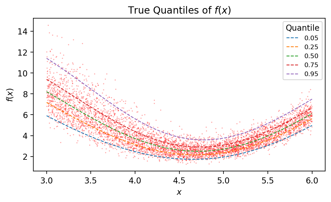
Below, 5000 points are generated according to the following function specification:

\[f(x) = (5.0 \cdot sin(x) + 7.5) \cdot \epsilon\]

\[\epsilon = lognormal \left( 0.0, \frac{1.0}{(x - 4.0)^2 + 4.0} \right)\]

# generate random data
def e(x):
    """Compute lognormal sigma as a function of x."""
    return 1.0 / ((x - 4.0) ** 2 + 4.0)

np.random.seed(17)
x = np.random.uniform(3.0, 6.0, size=5000)
error = np.random.lognormal(mean=0.0, sigma=e(x))
y = (5.0 * np.sin(x) + 7.5) * error

# plot true quantiles
fig = plt.figure(figsize=(6.5, 3.5), dpi=200)
ax = fig.add_subplot(111)
ax.scatter(x, y, s=0.1, color="red", alpha=0.5)

quantiles = [0.05, 0.25, 0.50, 0.75, 0.95]
xs = np.linspace(3.0, 6.0, 1001)
es = e(xs)
band_list = list()
for i, q in enumerate(quantiles):
    values = (5.0 * np.sin(xs) + 7.5) * scst.lognorm.ppf(q, es)
    band_list.append(values)
    ax.plot(xs, values, linestyle="--", linewidth=1.0, label=f"{q:0.2f}")

ax.legend(loc="best", title="Quantile", fontsize=8)
ax.set_ylabel("$f(x)$")
ax.set_xlabel("$x$")
ax.set_title("True Quantiles of $f(x)$");

Specify different modeling algorithms

Parameters here are arbitrary. There is no tuning or CV performed.

from sklearn.neural_network import MLPRegressor
from sklearn.tree import DecisionTreeRegressor
from sklearn.ensemble import RandomForestRegressor
from sklearn.gaussian_process import GaussianProcessRegressor
from sklearn.neighbors import KNeighborsRegressor

# create list of different model algorithm callbacks with some kwargs
# note: no tuning/CV has been done here
model_names = [
    "Neural Network",
    "Decision Tree",
    "Random Forest",
    "Gaussian Process",
    "KNeighbors Regressor",
]

model_list = [
    {
        "model_callback": MLPRegressor,
        "model_callback_kwargs": {"hidden_layer_sizes": (16, 8, 4),
                                  "max_iter": 1000,
                                  "alpha": 0.02,}
    },
    {
        "model_callback": DecisionTreeRegressor,
        "model_callback_kwargs": {"splitter": "random",
                                  "max_depth": 3,
                                  "min_samples_split": 25,}
    },
    {
        "model_callback": RandomForestRegressor,
        "model_callback_kwargs": {"n_estimators": 10,
                                  "min_samples_split": 30,
                                  "max_depth": 3,}
    },
    {
        "model_callback": GaussianProcessRegressor,
        "model_callback_kwargs": None
    },
    {
        "model_callback": KNeighborsRegressor,
        "model_callback_kwargs": {"n_neighbors": 100,}
    },
]

Fit the model ensembles

# fit models
model_results_list = list()
for i, (q, kwargs) in enumerate(zip(quantiles, model_list)):
    print("Fitting ensemble of {:s} models...".format(model_names[i]))
    model = BoostedModel(
        link=IdentityLink(),
        loss=QuantileLoss(q),
        weights="none",
        alpha=0.2,
        step_type="constant",
        validation_fraction=0.15,
        validation_iter_stop=20,
        **kwargs
    )
    model.fit(x.reshape((-1, 1)), y, iterations=500)
    preds = model.predict(xs.reshape((-1, 1)))
    model_results_list.append((model, preds))

Fitting ensemble of Neural Network models...
Fitting ensemble of Decision Tree models...
Fitting ensemble of Random Forest models...
Fitting ensemble of Gaussian Process models...
Fitting ensemble of KNeighbors Regressor models...

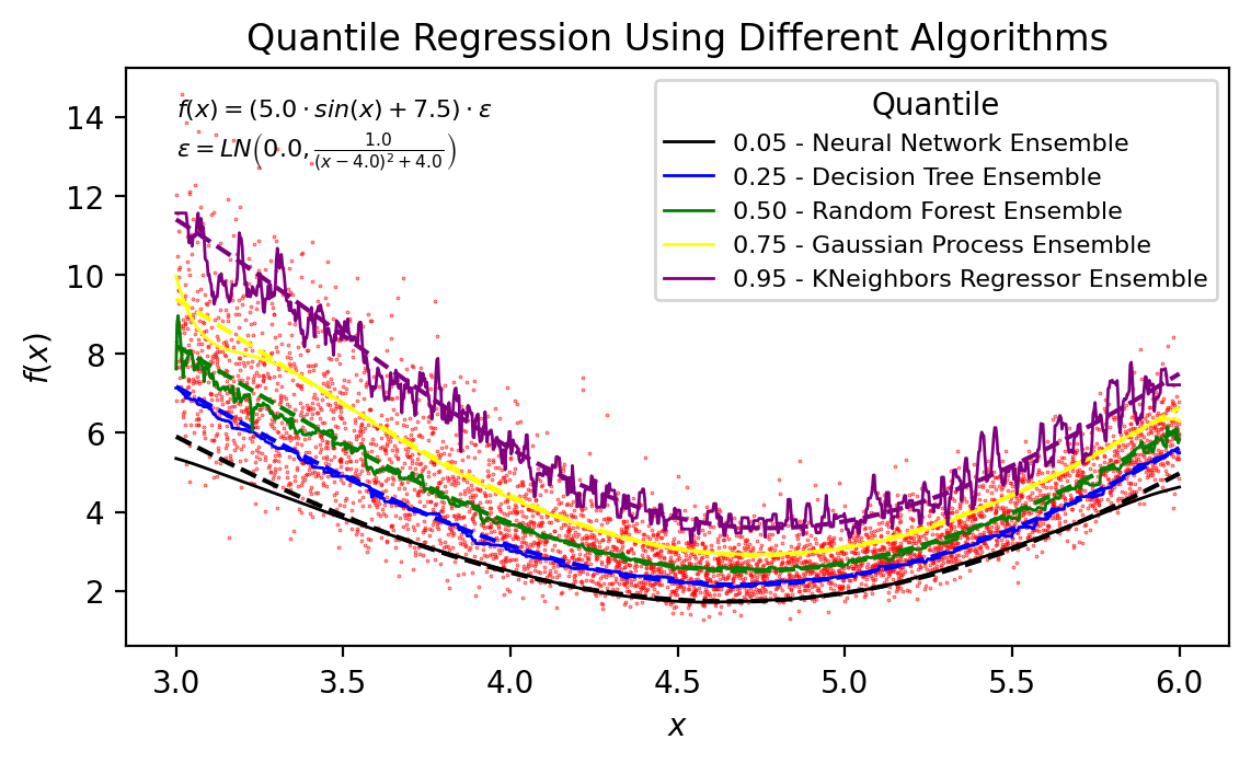
Plot the results

fig = plt.figure(figsize=(6.5, 3.5), dpi=200)
ax = fig.add_subplot(111)
ax.scatter(x, y, s=0.1, color="red", alpha=0.75)

colors = ["black", "blue", "green", "yellow", "purple"]
for i, (model, preds) in enumerate(model_results_list):
    q, model_name = quantiles[i], model_names[i]
    label = f"{q:0.02f} - {model_name} Ensemble"
    ax.plot(
        xs, band_list[i],
        color=colors[i],
        linestyle="--",
        label="__nolegend__"
    )
    ax.plot(xs, preds, color=colors[i], label=label, linewidth=1)
ax.legend(loc="best", title="Quantile", fontsize=8)
ax.set_ylabel("$f(x)$")
ax.set_xlabel("$x$")
ax.set_title("Quantile Regression Using Different Algorithms")
ax.text(3, 14,
        r"$f(x) = (5.0 \cdot sin(x) + 7.5) \cdot \epsilon$",
        fontsize=8,
)
ax.text(3, 13,
        r"$ \epsilon = LN \left( 0.0, \frac{1.0}{(x - 4.0)^2 + 4.0} \right) $",
        fontsize=8,
);

Model Iterations

for i, (model, preds) in enumerate(model_results_list):
    print("{:s}: {:d} iterations".format(model_names[i], model.get_iterations()))

Neural Network: 310 iterations
Decision Tree: 96 iterations
Random Forest: 94 iterations
Gaussian Process: 95 iterations
KNeighbors Regressor: 170 iterations